 - Download PDF-
SEEFOR 5 (2): 153-161
Article ID: 32
DOI: http://dx.doi.org/10.15177/seefor.14-17
Original scientific paper
Canopy Layers Stratified Volume Equations for Pinus caribaea Stands in South West Nigeria using Linear Mixed Models
Peter Oluremi Adesoye 1*
1 University of Ibadan, Faculty of Agriculture and Forestry, Department of Forest Resources Management, Ibadan, Nigeria
* Corresponding author: e-mail:
Citation:
ADESOYE PO 2014 Canopy Layers Stratified Volume Equations for Pinus caribaea Stands in South West Nigeria using Linear Mixed Models. South-east Eur for 5 (2): 153-161. DOI: http://dx.doi.org/10.15177/seefor.14-17
Received: 7 Oct 2014 / Accepted: 20 Nov 2014 / Published online: 13 Dec 2014
Cited by: CrossRef Google Scholar
Abstract
Background and Purpose: Efficient forest stand management requires reliable estimates of growing stock. The reliability of stem volume estimates depends on the range and extent of available sample data. The potentials of canopy layers stratification in pure plantations as a means of improving the accuracy of stem volume equations have not been fully explored. Linear Mixed Model (LMM) approach is a statistical technique capable of yielding a more efficient prediction under clustered data structure. This study investigates the existence and potentials of canopy stratifications for improving the reliability of stem volume prediction equations under pure plantations using linear mixed model approach.
Materials and Methods: Pinus caribaea Morelet plantations in Oluwa Forest Reserve, Ondo State, Nigeria were investigated. Individual tree growth variables, including diameters, heights and crown measurements were obtained in 2010 on twenty five 0.04 ha plots representing five different stands planted between 1979 and 1991. Visual assessment of the trees within each plot was also done to classify them into four canopy strata (i.e. dominant, co-dominant, intermediate and suppressed). Linear mixed model approach was used to analyze the tree growth data using SAS Proc Mixed. Two variants of volume equations; simple linear and exponential were investigated.
Results: Results show that simple linear mixed model consistently give better fit criteria (e.g. AIC) of 135.8, 18.9, -214.7 and -174.6 under dominant, co-dominant, intermediate and suppressed canopy layers, respectively. The covariance parameter estimate for dominant canopy (0.2219) is about 370 as large as that of suppressed (0.0006). This implies that canopy layers not only influence stem volume prediction but also reduce within-stand variance as well.
Conclusion: Simple linear mixed model produced better fitting criteria in terms of lower values of Akaike’s and Bayesian Information Criteria. Canopy stratification in pure stands of Pinus caribaea showed great potentials in improving the predictive ability of volume equations.
Keywords: stem volume equation, Pinus caribaea Morelet, dominant, co-dominant, intermediate, suppressed, linear mixed model
INTRODUCTION
Sustainable forest management requires reliable estimates of growing stock. Such information guides forest managers in timber evaluation as well as in the allocation of forest areas for harvest. For timber production, an estimate of growing stock is often expressed in terms of timber volume, which can be estimated from easily measurable tree dimensions. The most common procedure is to use volume equations based on relationships between stem volume and tree growth variables such as diameter and height. The reliability of volume estimates depends on the range and extent of the available sample data. In Nigeria, considerable work has been done on the development of volume equations for planted forests [1], [2], [3], [4], [5]. However, the effects of canopy layers on volume equations have not been fully investigated.
Classifications of individual trees into crown classes on the basis of their relative dominance in a stand have been made for many years. Four classes (i.e. dominant, co-dominant, intermediate and suppressed) are commonly recognized in forest ecology [6], [7]. Crown classification has been useful for predicting mortality, assessing tree vigour and rating tree resistance to certain diseases. However, for most pure plantations, the potentials of canopy layers for improving the accuracy of volume equations have not been fully explored. It has been established that when competition occurs between trees in even-aged stands or even-aged groups the trees begin to differentiate into crown classes.
A number of modeling techniques have been used for modeling stem volumes ranging from stand levels to individual tree approach. An important area that has been consistently overlooked is the fact that stem volume data are generally taken from trees growing in plots, located in different stands and of course under different canopy layers. This hierarchical structure usually results in a lack of independence between observations. This consequently results in biased estimates for the confidence interval of parameters if ordinary least squares regression techniques are used. To deal with this problem, mixed model approaches have been introduced.
Linear mixed model approach is a statistical technique generating improvements in parameter estimation. The approach has been used in many fields of study for nearly more than twenty years. However, in forestry, studies using mixed effects models are relatively recent. Lappi and Bailey [8] described the use of non-linear mixed effects growth curve based on Richards’s model. The model was fitted to predict dominant and co-dominant tree height, both at plot and individual tree levels. Gregoire et al. [9] studied linear mixed effects modeling of the covariance among repeated measurements with random plot effects. Zhang and Borders [10] used the mixed effects modeling method to estimate tree compartment biomass for intensively managed loblolly pine stands in USA. Fehrmann et al. [11] used mixed effects modeling to establish single-tree biomass equations for Norway spruce and Scots pine. Furthermore, application of linear mixed models was investigated in many other studies [e.g. 12], [e.g. 13], [e.g. 14], [e.g. 15], [e.g. 16], [e.g. 17], [e.g. 18]. Mixed effects models estimate both fixed and random parameters simultaneously for the same model. This results in consistent estimates of the fixed parameters and their standard errors. Furthermore, the inclusion of random parameters captures more variation among and within individuals or subjects.
Linear mixed models are capable of predicting random plot or tree effects unlike ordinary regression models. Hence, they are capable of yielding a more efficient prediction. Linear mixed models also allow for the explicit separation of the between and within canopy layers relationships and thus have the potentials for a correct specification of the model. The objectives of this study were to: (i) develop volume equations for Pinus caribaea Morelet (Pine) in south west Nigeria based on linear mixed modeling approach; (ii) determine and account for variance-covariance structure within individual trees; and (iii) evaluate the predictability of mixed model based on the calibration.
MATERIALS AND METHODS
Field Data
Field data were obtained from Pine stands in Oluwa Forest Reserve, Ondo state, Nigeria. The reserve lies between latitudes 6o 35’ and 7o 00’ North and longitudes 4o 25’ and 4o 55’ East. The Pine stands in Oluwa Forest Reserve were established around two local communities namely, Epe-makinde (comprising of 1989, 1990 and 1991 stands) and Omotosho along Lagos-Ore road (comprising of 1979 and 1980 stands). Figure 1 shows the map of Oluwa Forest Reserve with the study locations.
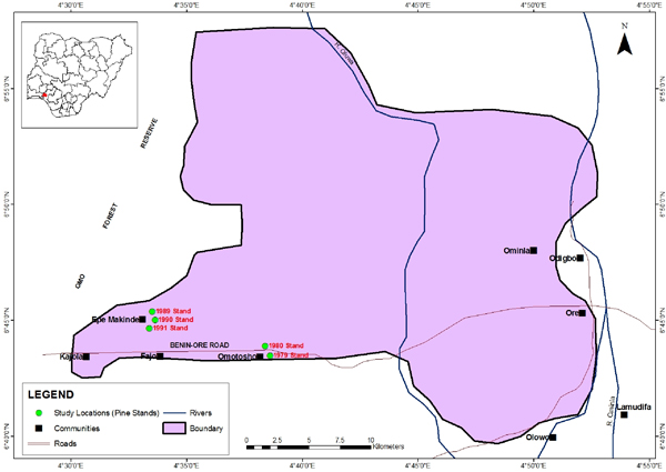
FIGURE 1. Map of Oluwa Forest Reserve showing the study locations
The stands were planted with initial spacing of 2 m x 3 m. There was no record of thinning in the stands. Majority of the soils in the Forest Reserve are representative of soils in the Ondo Association. These comprise of well drained, mature, red stony and gravely soils in the upper parts of the sequence, grading into the hill wash overlying original parent material or hardpan layers in the valley bottom [19]. The texture of the topsoil in the Reserve is sandy loam, which gradually becomes heavier as soil depth increases. The sub soils consist largely of clay with gravel occurring at 30-60 cm depth. According to Orwa et al. [20], Pine grows best in frost-free areas up to about 700 m altitude in more fertile sites with good subsoil drainage and annual rainfall of 2000-3000 mm. Soil requirements for Pine is usually loams or sandy loams. In some cases high amount of gravel and generally well drained soils have proved suitable. The soil ph is usually between 5.0 and 5.5. The species is rated as moderately fire resistant. It tolerates salt winds and hence may be planted near coast.
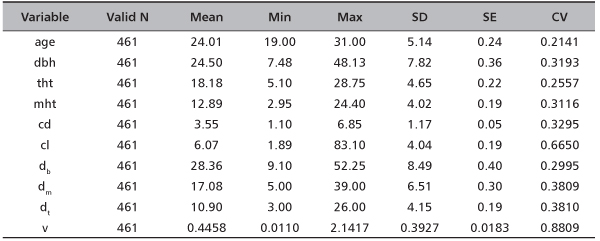
Data were collected from Pine stands established in 1979, 1980, 1989, 1990, and 1991. Five temporary sample plots of size 20 m x 20 m were randomly laid in each of the stand ages. Within each plot, tree growth variables, including diameter at breast height, base, middle and top (merchantable limit), total and merchantable heights, crown length and diameter were obtained in 2010. In addition, visual assessment of the trees within each plot was also done to classify them into four canopy layers (i.e. dominant, co-dominant, intermediate and suppressed). Individual stem volume was computed using the Newton’s formula. This is given as

where v is stem volume; mht is merchantable height; Ab, Am and At are cross sectional areas at the base, middle and top; db, dm and dt arediameters at the base, middle and top. Table 1 gives the summary statistics of the measured and derived variables at individual tree level.
TABLE 1. Summary statistics of the measured and derived variables of Pine at individual tree level
Linear Mixed Model Specification
A mixed model is constructed by incorporating a random component, denoted by zu, into the conventional formula of a linear model given by y = Xβ + ε . Using a matrix notation, a linear mixed model (LMM) can be written as follows:
Y = Xβ + Zu + ε
where Y is the vector of measurement of the study variable, Xβ is the fixed part of the model (similar to the standard linear models) such that X denotes the (n x p) observation or design matrix and β denotes the unknown (p x 1) vector of fixed intercept and slope effects of the model. Zu+ε is the random part, where u is a (q x 1) vector of random intercept and slope effects with an assumed q-dimensional normal distribution with zero expectation and (q x q) covariance matrix denoted by G and Z is the (n x q) design matrix of the random effects. Note that the structure of the covariance matrix G is not specified. The residuals ε can be correlated and the possibly non-diagonal covariance matrix of the residuals is denoted by R. A key assumption for linear mixed model is that u and ε are normally distributed such that
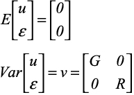
where G is the variance – covariance matrix of U and R is the variance – covariance matrix ε. The variance of the response variable y is V = ZGZT + R and can be estimated by setting up the random – effects design matrix Z and by specifying covariance structure for G and R. If R is specified as a diagonal matrix, LMM only considers the random effects such as blocks which can be reflected by G. Thus, the LMM with diagonal R and a specific G is normally called as the LMM block model.
For the purpose of model prediction, it is required not only to estimate the parameters of the fixed and covariance, but also to estimate the random effects. The solutions for β and u in LMM are called the best linear unbiased predictor (BLUP). In the LMM the fixed-effect parameters, β and the covariance parameters, θ (i.e. θG and θR for the G and R, matrices, respectively) are estimated. Note that by definition, random effects are random variables. Assume that the q random effects in the ui vector follow a multivariate normal distribution, with mean of vector 0 and a variance - covariance matrix denoted by D. Usually, the maximum likelihood (ML) and restricted maximum likelihood (REML) estimation methods are commonly used to estimate these parameters. In general, ML estimation is a method of obtaining estimates of unknown parameters by optimizing a likelihood function [21]. The REML is an alternative way of estimating the covariance parameters in θ. REML is sometimes called residual maximum likelihood estimation. It is often preferred to ML estimation, because it produces unbiased estimates of covariance parameters by taking into account the loss of degree of freedom that results from estimating the fixed effects in β.
Model Assessment
Akaike’s Information Criterion (AIC) and Bayesian Information Criterion (BIC) are commonly used for model selection and comparison [22]. The AIC may be calculated based on the ML or REML log-likelihood, l ( β, θ), of a fitted model as follows:

where L is likelihood, p is the number of fixed effect terms and k is the number of random effect terms. The candidate model with the lowest AIC is selected as the best model. The BIC may be calculated as follows:

The BIC applies a greater penalty for models with parameters than does the AIC, because the number of parameters being estimated is multiplied by the natural logarithm of n, where, n is the total number of observations used in estimation of the model. It has been suggested that no one information criterion stands apart as the best criterion to be used when selecting LMM and that more work still needs to be done in understanding the role that information criteria play in the selection of LMM [23].
Furthermore, likelihood ratio test (LRT) has been used extensively as a tool for testing the significance of random effects in LMM. To test the significance of one random effect, it assumes the effect has zero variance in the null hypothesis. Thus, the test statistic of LRT is defined as:

where θREML,0 and θREML,1 are restricted maximum likelihood estimates under the null-hypothesis and under the alternative hypothesis respec-tively [24]. The statistic -2lnλn follows a x2 distribution with degrees of freedom equal to the difference of the number of parameters of random effects in the model under the null and alternative hypotheses.
Model Implementation
In this study, a close investigation of the scatter plot of the stem volume (v) against diameter at breast height (dbh) revealed approximately a curvilinear shape. Therefore, two functional forms of tree v – dbh relationship (i.e. simple linear and exponential models) were investigated under the four canopy layers using linear mixed model approach. The model forms are as follows:
![]()

where ln is natural logarithm, β0 and β1 are regression coefficients to be estimated and ε is the model error term. Model residuals are defined as the difference between the observed and the predicted stem volume.
RESULTS
Model Fitting
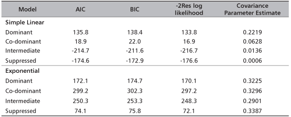
Table 2 indicates that simple linear mixed models consistently had significant improvement over the exponential models under the four canopy layers. Both AIC and BIC are consistently lower in simple linear mixed models across the canopy layers. Table 2 also displays the covariance parameter estimates. The covariance estimate for dominant canopy layer (0.2219) under simple linear mixed model is about 370 times larger than that of the suppressed canopy (0.0006). This implies that canopy layers not only have significant influence on stem volume prediction but also reduce their within-stand variances as well. The covariance parameter estimates for the different canopy layers under the exponential model do not show any definite order. This further confirms the non suitability of the equations.
TABLE 2. Model fitting statistics under the two modeling approaches across the crown layers
Model Coefficients of Fixed Effects
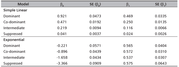
The estimates of coefficients of fixed effects and standard error (SE) of estimates of the models across the crown layers are presented in Table 3. Both the simple linear and exponential models produce significant main effects (p<0.0001). The standard error values generally are low. However, under the simple linear mixed models the standard error values are lower and also show a decreasing order from dominant canopy to suppressed canopy layer. This implies better fit.
TABLE 3. Estimates of model coefficients and standard errors (SE) of the fixed effects
DISCUSSION
The results obtained in this study have demonstrated that LMM has the capacity to improve volume equations under different canopy layers. The simple linear model approach produced better models judging from the lower values of AIC and BIC in contrast with the exponential models. This agrees with past studies [e.g. 25]. However, it is noteworthy that LMM with better fitting does not necessarily produce better model prediction [26].
Crown layer stratification has demonstrated the potentials to improve stem volume – dbh relationship. This is evident from the consistent lower standard error values in the models across the canopy layers. This finding confirms the assertions from previous studies [e.g. 27], [e.g. 28] of the existence and influence of canopy layers. The use of linear mixed models was designed to deal with the spatial heterogeneity in the data. Thus it produced more reliable estimates of fixed effects and smaller intra block variances of residuals (indicating the reduction of spatial heterogeneity in model residuals).
One area that obviously requires further study is the aspect of evaluating the influence of different covariance structure specification on the LMM with canopy stratification.
CONCLUSIONS
In this study, two variants of canopy layers stratified volume equations were investigated using linear mixed model approach (i.e. simple linear and exponential models) for Pinus caribaea stands in Oluwa Forest Reserve. The results indicated that, in general, simple linear mixed models produced better fit judging from the significantly reduced information criteria. This is an indication that LMM has the capacity to address effectively, spatial heterogeneity often encountered in forest growth data. The study also demonstrated the potentials of canopy layer stratification in improving volume prediction. Future work is required to focus on investigating the influence of different covariance structure specifications on the LMM performance.
Furthermore, recent studies suggest that better model fitting does not necessarily imply better prediction. This also requires further study to ascertain this claim.
REFERENCES
- OKOJIE JA, NOKOE S 1976 Choosing appropriate volume equations for Gmelina arborea (Linn.) for two plantation sites in Nigeria. Nigerian Journal of Forestry 6 (1-2): 67-69
- ABAYOMI JA 1983 Volume tables for Nauclea diderrichii in Omo Forest Reserve Nigeria. Nigerian Journal of Forestry 13 (1-2): 46-52
- OSHO JSA 1983 Volume prediction from stump diameter for teak (Tectona grandis F.) in Onigambari Forest Reserve. Nigerian Journal of Forestry 13: (1-2): 53-56
- AKINDELE SO 1987 Appropriate function for estimating tree volumes from stump diameters. Obeche 20-21: 4-10
- ONYEKWELU JC, AKINDELE SO 1995 Stand volume equations for Gmelina arborea plantations in Oluwa Forest Reserve Nigeria. Nigerian Journal of Forestry 24-25: 92-95
- JOHNSON PS, SHIFLEY SR, ROGERS R 2002 The Ecology and Silviculture of Oaks. CAB International, Wallingford, United Kingdom, 489 p. DOI: http://dx.doi.org/10.1079/9780851995700.0000
- CLARK DA, CLARK DB 1992 Life history diversity of canopy and emergent trees in a Neotropical rainforest. Ecol Monogr 62 (3): 315-344. DOI: http://dx.doi.org/10.2307/2937114
- LAPPI J, BAILEY RL 1988 A height prediction model with random stand and tree parameters: an alternative to traditional site index methods. Forest Sci 34 (4): 907-927
- GREGORIE TG, SCHABENBERGER O, BARRETT JP 1995 Linear modeling of irregularly spaced unbalanced, longitudinal data from permanent plot measurements. Can J Forest Res 25 (1): 137-156. DOI: http://dx.doi.org/10.1139/x95-017
- ZHANG YJ, BORDERS BE 2004 Using a system mixed effects modeling method to estimate tree compartment biomass for intensively managed loblolly pines – an allometric approach. Forest Ecol Manag 194 (1-3): 145-157. DOI: http://dx.doi.org/10.1016/j.foreco.2004.02.012
- FEHRMANN L, LEHTONEN A, KLEINN C, TOMPPO R 2008 Comparison of linear and mixed–effect regression models and a k-nearest neighbor approach for estimation of single-tree biomass. Can J Forest Res 38 (1): 1-9. DOI: http://dx.doi.org/10.1139/X07-119
- GREGORIE TG, SCHABENBERGER O 1996 Nonlinear mixed – effects modeling of cumulative bole volume with spatially correlated within-tree data. J Agric Biol Envir S 1 (1): 107-119. DOI: http://dx.doi.org/10.2307/1400563
- FANG Z, BAILEY RL 2001 Nonlinear mixed effects modeling for slash pine dominant height growth following intensive silvicultural treatments. Forest Sci 47 (3): 287-300
- JIANG L, LI F 2008 Modeling tree diameter growth using nonlinear mixed – effects models. In: Tan H, Wu B (eds) Proceedings of International Seminar on Future Information Technology and Management Engineering, Leicestershire, United Kingdom, 20 November 2008. IEEE Computer Society, Los Alamitos, California, USA, pp 636-639. DOI: http://dx.doi.org/10.1109/FITME.2008.141
- LANG P 2008 Linear mixed model of aerial photo crown width and ground diameter. Sci Silvae Sin 44 (3): 41-44
- LEI X, LI Y, XIANG W 2009 Individual basal area growth model using multi-level linear mixed model with repeated measurements. Sci Silvae Sin 45 (1): 74-80
- JIANG L, LI Y 2010 Application of nonlinear mixed – effects modeling approach in tree height prediction. Journal of Computers 5 (10): 1575-1581. DOI: http://dx.doi.org/10.4304/jcp.5.10.1575-1581
- LI C, ZHANG H 2010 Modeling dominant height for Chinese fir plantations using a nonlinear mixed effects modeling approach. Sci Silvae Sin 46 (3): 89-95
- SMYTH AJ, MONTGOMERRY RF 1962 Soils and Land Use in Central Western Nigeria. Government Printer, Ibadan, Nigeria, 265 p
- ORWA C, MUTUA A, KINDT R, JAMNADASS R, ANTHONY S 2009 Agroforestry Database: A Tree Reference and Selection Guide Version 4.0. World Agroforestry Centre, Kenya. URL: http://www.worldagroforestry.org/sites/treedbs/treedatabases.asp (17 September 2014)
- CASELLA G, BERGER RL 2002 Statistical inference. Duxbury, Pacific Grove, California, USA, 660 p
- HOETING JA, DAVIS RA, MERTON AA, Thompson SE 2006 Model selection for geostatistical models. Ecol Appl 16 (1): 87-98. DOI: http://dx.doi.org/10.1890/04-0576
- GURKA MJ 2006 Selecting the best linear mixed model under REML. Am Stat 60 (1): 19-26. DOI: http://dx.doi.org/10.1198/000313006X90396
- VERBEKE G, MOLENBERGERGHS G 1997 Linear mixed models in practice. Lecture Notes in Statistics 126: 63-153. DOI: http://dx.doi.org/10.1007/978-1-4612-2294-1_3
- ZHANG L, GOVE JH, HEATH LS 2005 Spatial residual analysis of six modeling techniques. Ecol Model 186 (2): 154-177. DOI: http://dx.doi.org/10.1016/j.ecolmodel.2005.01.007
- LU J, ZHANG L 2013 Evaluation of structure specification in linear mixed models for modeling the spatial effects in tree height-diameter relationships. Ann For Res 56 (1): 137-148
- PARKER GG, BROWN MJ 2000 Forest Canopy Stratification – Is It Useful? Am Nat 155 (4): 473-484. DOI: http://dx.doi.org/10.1086/303340
- ISHII H, REYNOLDS JH, FORD ED, SHAW DC 2000 Height growth and vertical development of an old-growth Pseudotsuga-Tsuga forest in southwestern Washington State, U.S.A. Can J Forest Res 30 (1): 17-24. DOI: http://dx.doi.org/10.1139/x99-180
© 2015 by the Croatian Forest Research Institute. This is an Open Access paper distributed under the terms of the Creative Commons Attribution License (http://creativecommons.org/licenses/by/4.0).

